How Much Does an A/B Test Really Cost?

What does it cost to run an A/B test?

The obvious answer is the cost of producing it.

Someone needs to research the problem, define a hypothesis, design the variation, build it, configure the experiment, test the tracking, run QA, monitor the results, and interpret what happened.

If an agency handles the work, there is an agency fee. If an internal team handles it, there are salaries and the opportunity cost of time that could have been spent elsewhere.

All of these costs are real.

But they are only the costs you can see before the experiment launches.

Once traffic starts flowing into the experiment, another kind of cost begins accumulating. It does not appear on an invoice. It is rarely included in the project estimate. Many experimentation platforms do not show it directly.

To understand that cost, we need to stop thinking of traffic as free.

Key takeaways

• A/B tests have operational costs and traffic-related opportunity costs.
• An inferior variation costs conversions while it continues receiving traffic.
• Expected conversions should be based on what the same traffic would likely have produced in Control.
• The calculation should be cumulative, not based on isolated daily differences.
• A stopped variation should remain anchored to the Control rate from when its traffic stopped.
• Eligible late conversions can still change the result after traffic stops.
• A loss budget is a business risk limit, not a statistical stopping rule.
• We built a PostHog dashboard to calculate this continuously for every variation.

The visible cost of running an A/B test

Before discussing lost conversions, we should acknowledge the costs most teams already budget for.

Research and strategy

A useful experiment starts before anyone opens a design tool.

The team may need to:

• Review analytics and funnel performance.
• Watch session recordings.
• Study customer research.
• Inspect previous experiments.
• Identify a bottleneck.
• Prioritize competing hypotheses.
• Define the expected mechanism behind the change.

Weak research produces weak tests, so this is not optional overhead.

Design and copy

The variation may require:

• New copy.
• Interface design.
• Responsive layouts.
• Product imagery.
• Prototypes.
• Stakeholder review.
• Legal or compliance review.

A minor copy test may take a few hours. A pricing, onboarding, or checkout experiment can involve several teams.

Development and implementation

Someone has to build the variation and ensure that each participant sees the correct experience.

Depending on the experiment, this may involve:

• Frontend code.
• Backend logic.
• Feature flags.
• CMS changes.
• Experiment-platform configuration.
• Identity handling.
• Variation persistence.
• Rollback logic.

Analytics and tracking

The primary outcome, secondary metrics, exposure event, conversion window, filters, and internal-traffic exclusions must be defined correctly.

If the metric is wrong, the experiment may be implemented perfectly and still produce an unusable answer.

Quality assurance

Every variation should be checked across:

• Mobile and desktop.
• Browsers and devices.
• Logged-in and logged-out states.
• Traffic sources.
• Markets or languages.
• Purchase and checkout paths.
• Analytics events.
• Error states.

Monitoring and analysis

After launch, someone must monitor traffic allocation, tracking integrity, technical errors, guardrail metrics, and eventual experiment results.

These costs matter. For a low-traffic business or an organization starting its first experimentation program, they may represent most of the cost.

But the economics change as traffic grows.

Traffic is part of the experimentation budget

An A/B test does not create new visitors for the variation. It redirects some of the business’s existing traffic away from Control.

That traffic would have produced some number of purchases, subscriptions, qualified leads, or other conversions if it had remained in Control.

When a variation performs better, the business may gain conversions.

When a variation performs worse, the business gives up conversions in exchange for information.

That exchange is a normal part of experimentation. You cannot learn whether a change is better without exposing some people to it.

The problem begins when the cost of that learning is not measured.

A weak variation can continue receiving thousands of visitors while the team waits for a result. On a high-volume funnel, a modest conversion-rate difference can become more expensive than the research, design, development, analytics, and agency work combined.

This is the opportunity cost of experimentation.

What is the opportunity cost of an A/B test?

The opportunity cost of an underperforming variation is the number of conversions the business would likely have received if the variation’s traffic had been sent to Control instead.

The underlying question is:

How many conversions did this traffic produce, and how many would we have expected from the same traffic under Control?

The first number is observed.

The second number must be estimated from the concurrent Control group.

The difference gives us the variation’s conversion impact.

How to calculate expected conversions

For a variation at a particular point in the experiment:

Expected conversions

= cumulative variation participants × comparable Control conversion rate

The signed conversion impact is:

Conversion impact

= actual variation conversions – expected conversions

Interpretation:

• A negative result means the variation has produced fewer conversions than expected.
• A positive result means the variation has produced more conversions than expected.
• Zero means the variation is at break-even relative to Control.

If you want to express only the downside:

Foregone conversions

= MAX(0, expected conversions – actual conversions)

We prefer retaining the signed result in the monitoring dashboard. Positive performance can then offset earlier negative performance, giving the team a cumulative conversion balance rather than a loss-only counter.

A practical example

Suppose an experiment has these cumulative results:

Metric	Control	Variation
Participants	20,000	20,000
Conversion rate	5.0%	4.5%
Actual conversions	1,000	900

If the variation’s 20,000 participants had converted at the 5% Control rate, we would have expected:

20,000 × 5% = 1,000 conversions

The variation actually produced 900:

900 – 1,000 = -100 conversions

The variation has therefore consumed 100 conversions of the experiment’s loss budget.

If an average conversion produces €100 in revenue, the rough gross-revenue difference would be €10,000.

But that financial translation is only defensible when conversion value is reasonably stable. If order values, margins, refunds, subscriptions, or customer quality vary by variation, the business needs a separate revenue or profit model.

The cleaner operational result is:

This variation has produced 100 fewer completed conversions than we would have expected from the same traffic in Control.

Why the calculation should be cumulative

Daily conversion rates are noisy.

Control may perform unusually well on Monday and unusually poorly on Tuesday. A variation can appear disastrous for a few hours and recover as more data arrives.

If we calculate the cost from each day in isolation, the dashboard will react too strongly to random daily movement.

A cumulative calculation is more stable:

Cumulative expected conversions

= cumulative variation participants × cumulative comparable Control rate

Then:

Cumulative impact

= cumulative actual conversions – cumulative expected conversions

As the experiment collects more data, the Control rate becomes more stable. A single unusual day has less influence on the total.

This does not eliminate uncertainty. It gives the team a more useful operational signal than comparing isolated calendar days.

Positive performance should offset negative performance

A loss-only metric can create the impression that every early shortfall is permanent.

Suppose a variation begins 12 conversions below expectation but later recovers and finishes five conversions above expectation. Its current cumulative impact should be +5, not −12.

The metric should reflect all information available at the current point:

Current cumulative balance

= all actual conversions so far – all expected conversions so far

The same principle applies across several variations when calculating overall experiment impact.

One variation may consume part of the loss budget while another creates incremental conversions. The overall result should be the sum of each variation’s signed impact.

However, each variation must first be compared with the correct Control benchmark. You should not pool all variation traffic and multiply it by one convenient Control rate when variations were active for different periods.

Why Control should be measured at the same point in time

Conversion rates change during an experiment.

A promotion may start. Traffic sources may shift. Weekday and weekend behavior may differ. The Control rate after three weeks may not match the Control rate after one week.

An active variation should therefore be compared with cumulative Control performance over the same stage of the experiment.

In plain language:

Compare variation traffic with the Control experience that existed while that variation was receiving traffic.

This keeps the estimate concurrent. It reduces the risk of attributing an external change in traffic or market conditions to the variation.

What happens when a variation is stopped early?

When a variation stops receiving traffic, its comparison with Control should also stop moving forward.

Suppose Variation A is stopped on day 10, while Control and Variation B continue until day 25.

Variation A should not be recalculated using Control’s day-25 conversion rate. It had no traffic during days 11 through 25 and was not exposed to the conditions affecting Control during that period.

Instead:

1. Stop adding new participants to Variation A.
2. Anchor its Control benchmark to cumulative Control performance on day 10.
3. Keep that benchmark fixed.
4. Continue counting eligible late conversions from people already assigned to Variation A.

This is the stopped-variation anchoring rule.

Without this rule, a stopped variation’s estimated cost can continue changing because of traffic conditions it never experienced.

Conversion windows still matter after traffic stops

Not every conversion happens immediately after exposure.

Someone may see a variation today and purchase tomorrow. A B2B lead may submit a form today and qualify several days later. A subscription may not generate its first payment until after a trial.

The experiment’s conversion window defines how long an outcome can be attributed to an exposure.

When a variation stops:

• No new participants should enter it.
• Participants already exposed may still convert.
• Eligible late conversions should continue updating the variation.
• The result becomes final only after the remaining attribution windows close.

Stopping traffic and stopping outcome observation are different decisions.

This is also why recent experiment data can change. A dashboard may include the latest exposure immediately while conversions continue arriving later.

The metric should use the latest available information

Opportunity cost is most useful as an operational measure.

A report based only on completed calendar days can miss what is happening during the current day. If a variation is rapidly losing purchases this morning, the team should not have to wait until tomorrow to see it.

A monitoring dashboard should therefore use the latest available data, including the current partial day, while making the freshness of that data clear.

The cumulative line may move as:

• New participants enter.
• New Control conversions occur.
• New variation conversions occur.
• Eligible late conversions arrive.
• A variation stops receiving traffic.

This continuous movement is expected. The dashboard represents the current estimate, not a permanently settled result.

What is an experiment loss budget?

An experiment loss budget is the maximum conversion downside the business is willing to tolerate while learning from a test.

It can be expressed as:

• A number of conversions.
• A percentage of normal conversion volume.
• A financial amount when conversion value is reliable.
• A separate threshold for each variation.
• An overall threshold for the complete experiment.

For example:

We are willing to risk up to 40 completed purchases while testing this hypothesis.

This does not mean the business expects to lose 40 purchases. It defines the point where continued exposure requires an explicit decision.

The appropriate budget depends on:

• Conversion value.
• Experiment importance.
• Expected learning.
• Traffic volume.
• Number of variations.
• Potential upside.
• Reversibility.
• Customer or operational risk.
• How quickly reliable evidence can accumulate.

A high-risk checkout experiment should usually have a tighter budget than a low-risk informational change far from purchase.

Set the loss budget before launch

A loss budget is most useful when it is agreed before anyone sees the results.

Otherwise, the threshold tends to move:

• A favored idea gets more time.
• A politically important variation receives special treatment.
• A noisy early loss causes panic.
• A nearly significant result encourages the team to tolerate more damage.
• The team stops only after someone notices the revenue decline elsewhere.

Before launch, document:

1. The business outcome being protected.
2. The maximum acceptable conversion loss.
3. Whether the limit applies per variation, overall, or both.
4. The conversion window.
5. Who reviews the dashboard.
6. What happens when the budget is consumed.
7. Which statistical stopping method governs winner decisions.

This turns loss tolerance into program governance rather than an improvised reaction.

A loss budget is not a statistical stopping rule

This is the most important limitation.

A variation appearing below Control does not automatically prove that it is harmful. Early experiment results can move substantially as more data arrives.

Likewise, repeatedly checking a conventional fixed-horizon significance result and stopping whenever the number looks favorable can inflate false-positive risk.

The loss budget answers a business question:

How much downside are we willing to tolerate while collecting evidence?

Statistical analysis answers a different question:

What does the experiment allow us to conclude about the variation’s effect?

Those questions should be designed together, but they are not interchangeable.

If the loss limit is reached, the team may:

• Pause the variation.
• Reduce its traffic.
• Investigate a technical problem.
• Review guardrail metrics.
• Stop exposure to protect the business.
• Continue only through a pre-agreed exception process.

Stopping for risk does not prove the variation has no value. The result may remain statistically inconclusive.

If you want repeated monitoring itself to produce formal statistical decisions, use a method designed for interim analysis or sequential testing. Do not bolt continuous peeking onto a fixed-horizon test and assume the inference remains unchanged.

Which conversion should the loss budget protect?

Use the completed business outcome you are unwilling to sacrifice.

For commerce, this is usually a completed purchase or successful payment.

For other businesses, it may be:

• A paid subscription.
• A qualified opportunity.
• An attended consultation.
• An approved application.
• A completed booking.
• A retained subscriber.

Avoid basing the loss budget entirely on an upstream event such as:

• Button clicked.
• Product viewed.
• Form started.
• Checkout opened.
• Pricing page visited.

An upstream event can improve while the final business outcome declines.

The protected metric should reflect the cost the organization actually cares about.

The loss budget is one half of CRO program measurement

A mature experimentation program needs two different views.

The first measures the cumulative impact of changes that were validated and deployed. We cover that in our companion guide on [measuring the cumulative impact of a CRO program].

The second measures the downside incurred while experiments are still running.

These views answer different questions:

Measurement	Question
Compounded uplift	What did our deployed experiment wins improve?
Experiment loss budget	How much conversion risk did we incur while finding those wins?

A program can produce strong deployed uplift while taking too much risk during testing. It can also control risk carefully but fail to deploy meaningful improvements.

Both sides matter.

Monitoring loss budgets in PostHog

Calculating this manually is possible, but maintaining it continuously is difficult.

The system must account for:

• Actual participants by variation.
• Actual completed conversions.
• Concurrent cumulative Control performance.
• Separate stop dates for each variation.
• Late conversions inside the attribution window.
• Positive and negative impact.
• Current partial-day data.
• Overall experiment impact.

If you use PostHog for experimentation, we have built an automated dashboard that handles these calculations for every variation.

The dashboard shows:

• The last traffic date for each variation.
• Cumulative participants.
• Actual completed purchases.
• Expected purchases based on Control.
• Relative performance versus Control.
• Purchases gained or lost.
• Overall experiment impact.
• A cumulative trend with a zero break-even line.

Stopped variations remain anchored to Control when their traffic ended, while eligible late purchases can still update their outcome.

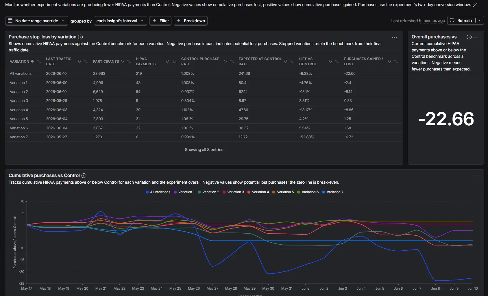
The dashboard does not decide whether an experiment should stop. It gives the team the information needed to apply its pre-agreed loss budget consistently.

A practical operating process

A loss-budget system works best as a short operating loop.

Before launch

• Confirm the protected business outcome.
• Verify the outcome tracking.
• Define the conversion window.
• Set per-variation and overall loss limits.
• Document the statistical decision method.
• Assign an owner.

While the experiment runs

• Monitor cumulative signed impact.
• Check whether losses are concentrated in one variation.
• Investigate technical or tracking anomalies.
• Confirm stopped variations are no longer receiving traffic.
• Apply the pre-agreed response when a threshold is reached.

After the experiment

• Allow eligible conversion windows to mature.
• Record why any variation was stopped.
• Separate risk decisions from statistical conclusions.
• Document the experiment’s final result and learning.
• Add deployed winners to the program’s compounded-uplift register.

Frequently asked questions

Treat conversion loss as an experiment resource

Losing conversions during an experiment is not automatically a failure.

It is part of the price of learning. The organization accepts a limited amount of uncertainty today in exchange for better decisions tomorrow.

But that does not mean the cost should be invisible or unlimited.

A mature experimentation program should know:

• How much it spends producing experiments.
• How much conversion risk each experiment creates.
• Which variations are consuming that risk.
• When the agreed loss limit has been reached.
• What the experiment has produced in return.

Team time is budgeted. Agency fees are budgeted. Development capacity is budgeted.

Traffic should be budgeted too.